Quantized conductance

The history of ballistic transport goes back to 1965, when Yuri Sharvin (Moscow) used a pair of point contacts to inject and detect a beam of electrons in a single-crystalline metal [4]. In such experiments the quantum mechanical wave character of the electrons does not play an essential role, because the Fermi wave length ( $\lambda_{\rm F}\approx 0.5\,{\rm nm}$) is much smaller than the opening of the point contact. The two-dimensional (2D) electron gas in a GaAs-AlGaAs heterojunction has a Fermi wave length which is a hundred times larger than in a metal. This makes it possible to study a constriction with an opening comparable to the wave length (and much smaller than the mean free path for impurity scattering). Such a constriction is called a quantum point contact.

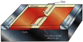
Figure 1. Schematic cross-sectional view of a quantum point contact, defined in a high-mobility 2D electron gas at the interface of a GaAs-AlGaAs heterojunction. The point contact is formed when a negative voltage is applied to the gate electrodes on top of the AlGaAs layer. Transport measurements are made by employing contacts to the 2D electron gas at either side of the constriction.

In a metal a point contact is fabricated simply by pressing two wedge- or needle-shaped pieces of material together. A quantum point contact requires a more complicated strategy, since the 2D electron gas is confined at the GaAs-AlGaAs interface in the interior of the heterojunction. A point contact of adjustable width can be created in this system using the split-gate technique developed in the groups of Michael Pepper (Cambridge) and Daniel Tsui (Princeton) [5]. The gate is a negatively charged electrode on top of the heterojunction, which depletes the electron gas beneath it. (See figure 1.) In 1988, the Delft-Philips and Cambridge groups reported the discovery of a sequence of steps in the conductance of a constriction in a 2D electron gas, as its width W was varied by means of the voltage on the gate [6,7]. (See PHYSICS TODAY, November 1988, page 21.) As shown in figure 2, the steps are near integer multiples of $2e^{2}/h\approx 1/13\,{\rm k}\Omega$ (after correction for a small gate-voltage independent series resistance).

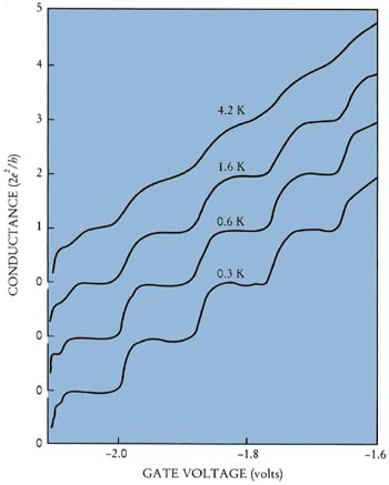
Figure 2. Conductance quantization of a quantum point contact in units of 2e²/h. As the gate voltage defining the constriction is made less negative, the width of the point contact increases continuously, but the number of propagating modes at the Fermi level increases stepwise. The resulting conductance steps are smeared out when the thermal energy becomes comparable to the energy separation of the modes. (Adapted from ref. [6].)

An elementary explanation of the quantization views the constriction as an electron wave guide, through which a small integer number $N\approx 2W/\lambda_{\rm F}$ of transverse modes can propagate at the Fermi level. The wide regions at opposite sides of the constriction are reservoirs of electrons in local equilibrium. A voltage difference V between the reservoirs induces a current I through the constriction, equally distributed among the N modes. This equipartition rule is not immediately obvious, because electrons at the Fermi level in each mode have different group velocities v_n. However, the difference in group velocity is canceled by the difference in density of states $\rho_{n}=1/hv_{n}$. As a result, each mode carries the same current $I_{n}=Ve^{2}\rho_{n}v_{n}=Ve^{2}/h$. Summing over all modes in the wave guide, one obtains the conductance G=I/V=Ne²/h. The experimental step size is twice e²/hbecause spin-up and spin-down modes are degenerate.

The electron wave guide has a non-zero resistance even though there are no impurities, because of the reflections occurring when a small number of propagating modes in the wave guide is matched to a larger number of modes in the reservoirs. A thorough understanding of this mode-matching problem is now available, thanks to the efforts of many investigators [8].

The quantized conductance of a point contact provides firm experimental support for the Landauer formula,

$$G=\frac{2e^{2}}{h}\sum_{n}t_{n},$$

for the conductance of a disordered metal between two electron reservoirs. The numbers t_n between 0 and 1 are the eigenvalues of the product ${\bf tt}^{\dagger}$ of the transmission matrix ${\bf t}$and its Hermitian conjugate. For an "ideal" quantum point contact Neigenvalues are equal to 1 and all others are equal to 0. Deviations from exact quantization in a realistic geometry are about 1%. This can be contrasted with the quantization of the Hall conductance in strong magnetic fields, where an accuracy better than 1 part in 10⁷ is obtained routinely [9]. One reason why a similar accuracy can not be achieved in zero magnetic field is the series resistance from the wide regions, whose magnitude can not be determined precisely. Another source of excess resistance is backscattering at the entrance and exit of the constriction, due to the abrupt widening of the geometry. A magnetic field suppresses this backscattering, improving the accuracy of the quantization.

Suppression of backscattering by a magnetic field is the basis of the theory of the quantum Hall effect developed by Marcus Büttiker (IBM, Yorktown Heights) [10]. Büttiker's theory uses a multi-reservoir generalization of the two-reservoir Landauer formula. The propagating modes in the quantum Hall effect are the magnetic Landau levels interacting with the edge of the sample. (Classically, these magnetic edge states correspond to the skipping orbits discussed later.) There is a smooth crossover from zero-field conductance quantization to quantum Hall effect, corresponding to the smooth crossover from zero-field wave guide modes to magnetic edge states.